MACRODEMOS

Macroeconomics Demos: A Python package to teach macroeconomics and macroeconometrics

The purpose of this package is to provide tools to teach concepts of macroeconomics and macroeconometrics.

To date, the package provides four functions:

ARMA_demo

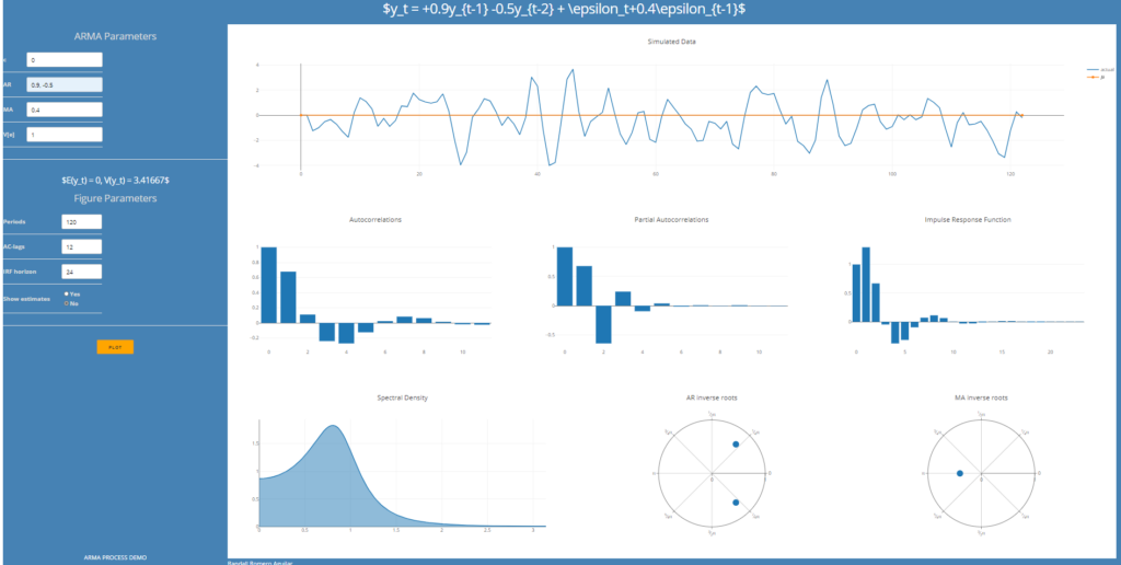
ARMA_demo is a tool for learning about ARMA processes. It creates a dash consisting of 7 plots to study the theoretical properties of ARMA(p, q) processes, as well as their estimated counterparts. The plots display

a simulated sample
autocorrelations
partial autocorrelations
impulse response function
spectral density
AR inverse roots
MA inverse roots.

filters_demo

filters_demo: The purpose of this demo is to help you understand several popular time series filtering methods:

Hodrick and Prescott (1997) Postwar U.S. Business Cycles: An Empirical Investigation
Baxter and King (1995) Measuring Business Cycles: Approximate Band-Pass Filters for Economic Time Series
Christiano and Fitzgerald (2003) The Band Pass Filter
Hamilton (2017) Why You Should Never Use the Hodrick-Prescott Filter
About the data

All data is quarterly, and is downloaded from the IFS database (IMF); for this reason, you need an Internet connection to run this demo. Furthermore, sometimes the IFS API will not return the requested data; in such case try again a few seconds later.

For each time series, this app downloads the nominal values in local currency and computes a real time series by dividing by the GDP deflator. The several filters are then applied to the logarithm of the resulting time series.

Countries shown in the dropdown menu are those for which there is data available in IFS.

Markov_demo

Markov_demo: a demo to illustrate Markov chains. User sets the number of states, the transition matrix, and the initial distribution. The demo creates a dash consisting of 2 plots:

a simulated sample
the time evolution of the distribution of states

Solow_demo

Solow_demo illustrates the Solow-Swan model. Users can simulate the dynamic effect of a shock in a exogenous variable or a change in a model parameter.

In the Simulations tab, you will find 6 figures simulating the adjustment paths to a change of variables or parameters:

Capital stock, per capita
Output per capita,
Savings per capita,
Consumption per capita,
Change in capital stock, and
Output growth rate

In the Equilibrium tab, you will see a diagram that illustrates how the steady-state equilibrium is reached.

In the Golden Rule tab, you will see how the capital stock, output, investment, and consumption (all in per capita terms) change in response to different savings rates.

Future of macrodemos

In a near future, I expect to add a few more demos:

Bellman_demo: to illustrate the solution of a Bellman equation by value function iteration
Filters_demo: to illustrate the use of the Hodrick-Prescott and the Baxter-King filters

Instructions

Option 1: The easiest way to run macrodemos is by opening the following Jupyter Notebook in Google colab: Macrodemos in Google Colab.ipynb

Option 2: To use the demos locally, just install the package

pip install macrodemos

and then in a Python session run (for example, to execute the ARMA_demo):

from macrodemos import ARMA_demo
ARMA_demo()

This will open a new tab in your default Internet browser with a Plotly dash.

Disclaimer

This program illustrates basic concepts of common tools used in analyzing macroeconomic data. It was developed for teaching purposes only. If you have any suggestions, please send me an email at [email protected]

macrodemos