DEMO: basis

This script provides examples on using the basisChebyshev class.

Last updated: October 4, 2014.

Copyright (C) 2014 Randall Romero-Aguilar

Licensed under the MIT license, see LICENSE.txt

Contents

EXAMPLE 2: Using basis and funcApprox to approximate a CobbDouglas function

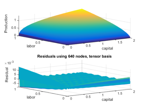
PROBLEM: Approximate the Cobb-Douglas production function y = f(K,L) = K^0.4 L^0.6 for capital K in [0,2] and labor L in [0,1].

y = @(K,L) K.^0.4 .* L.^0.6;

Using a tensor-product basis

Create a 2-D Chebyshev basis T by taking the tensor product of the individual dimensions

opts.type = 'cheb';
opts.method = 'tensor';
opts.nodetype = 'lobatto';
opts.varnames = {'capital','labor'};

T = basis([32 20],[0 0],[2 1],opts);
disp(T)

Basis of 2 dimension(s)

	    Variable           # of nodes       Interval    
	capital                    32       [  0.00,   2.00]
	labor                      20       [  0.00,   1.00]

	Type of basis:         cheb        
	Type of nodes:         lobatto     
	Expansion method:      tensor      
	Total basis nodes:     640         
	Total basis functions: 640         

The level of production at the collocation nodes is

yTnodes = y(T.nodes(:,1),T.nodes(:,2));

The approximated function, using basis T, is

yT = funcApprox(T,yTnodes);

Plot the functions

ngrid = 201;
kk = linspace(T.a(1),T.b(1),ngrid)';
ll = linspace(T.a(2),T.b(2),ngrid)';
[kk,ll] = meshgrid(kk,ll);

yy = y(kk,ll);
yTapprox = reshape(yT.Interpolate([kk(:),ll(:)]),ngrid,ngrid);

figure
subplot(2,1,1), surf(kk,ll,yy,'EdgeColor','none')
hold on
surf(kk,ll,yTapprox,'EdgeColor','none')
axis tight
xlabel(T.opts.varnames(1)), ylabel(T.opts.varnames(2)), zlabel('Production')


subplot(2,1,2), surf(kk,ll,yTapprox - yy,'EdgeColor','none')
title('Residuals using 640 nodes, tensor basis'), axis tight
xlabel(T.opts.varnames(1)), ylabel(T.opts.varnames(2)), zlabel('Residual')

Using a Smolyak basis

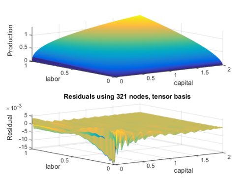
Now repeat the exercise with Smolyak nodes, with degree and node parameters set to q = 3. Call the basis S

opts.method = 'smolyak';
opts.degreeParam = 6;
opts.nodeParam = 6;

S = basis([80 50],[0 0],[2 1],opts);
disp(S)

Notice the warning about the number of Smolyak nodes: The number of nodes for each dimension must be n = 2^k+1 for some positive integer k. If user calls the constructor with different number of nodes, the constructor increases n to the next admissible value (from 80 to 129 for capital, and from 50 to 65 for labor).

Warning: For Smolyak expansion, number of nodes should be n=2^k + 1,for some k =
1,2,... 
Adjusting number of nodes
	 Old n,  New n
	    80,    129
	    50,     65

Basis of 2 dimension(s)

	    Variable           # of nodes       Interval    
	capital                    129      [  0.00,   2.00]
	labor                      65       [  0.00,   1.00]

	Type of basis:         cheb        
	Type of nodes:         lobatto     
	Expansion method:      smolyak     
	Total basis nodes:     321         
	Total basis functions: 321         

The level of production at the new collocation nodes is

ySnodes = y(S.nodes(:,1),S.nodes(:,2));

The approximated function, using basis S, is

yS = funcApprox(S,ySnodes);

Plot the functions

ySapprox = reshape(yS.Interpolate([kk(:),ll(:)]),ngrid,ngrid);

figure
subplot(2,1,1), surf(kk,ll,yy,'EdgeColor','none')
hold on
surf(kk,ll,ySapprox,'EdgeColor','none')
axis tight
xlabel(S.opts.varnames(1)), ylabel(S.opts.varnames(2)), zlabel('Production')


subplot(2,1,2), surf(kk,ll,ySapprox - yy,'EdgeColor','none')
title('Residuals using 321 nodes, tensor basis'), axis tight
xlabel(S.opts.varnames(1)), ylabel(S.opts.varnames(2)), zlabel('Residual')

Notice that the residuals in Smolyak and tensor bases are of similar magnitude, despite the fact that Smolyak is using around half the number of nodes and bases functions (i.e., its interpolation matrix is around one-forth the size of the tensor interpolating matrix).

Published with MATLAB® R2014b